Graph
Introduction of Graph
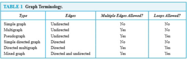
Definition of Graph
Multigraphs
Pseduographs
Directed Graphs
Directed Multigraphs
Graphs Models
Graph Terminology
We will learn the following terms:
- Adjacent
- connect
- endpoint
- neighborhood
- degree
- initial
- terminal
- in-degree
- out-degree
- complete
- cycles
- wheels
- n-cubes
- bipartite
- subgraph
- union
Special Types of Graphs
Bipartite Graphs
New Graphs from Olds
Graph Representation & Isomorphism
Graph Representation
Adjacency List
Adjacency Matrices
Incidence Matrices
Graph Isomorphism
Connectivity
Path
In a undirected graph, a path of length from to is a sequence of adjacent edges going from vertex to .
- A path is a circuit , or close walk, if
- A path traverses then vertices along it
- A path is simple if it contains no edge more than once. When a path is simple, we can denote this path by these vertices sequence
Path in Directed Graphs
Same as in undirected graphs, but the path must go in the direction of the arrows.
- When there are no multiple edged in the directed graph, this path is denoted by its vertices sequence same as that in undirected graph
- A path of length greater than zero and begins and ends at the same vertex is called a circuit or cycle
Connectedness
An undirected graphs is connected if there is a path between every pair of distinct vertices in the graph. An undirected graph that is not connected is called disconnected. We say that we disconnect a graph when we remove vertices or edges, or both, to produce disconnected subgraph.
Theorem: There is a simple path between any pair of vertices in a connected undirected graph.
Cut Vertices & Cut Edge
We call a connected graph is a connected component
- The removal from a graph of a vertex and all incident edges produces a subgraph with more connected components. Such vertices are called cut vertices or articulation points.
- An edge whose removal produces a graph with more connected components than in the original graph is called a cut edge or bridge.
- A cut vertex or cut edge separates 1 connected component into 2 if removed.
Vertex Connectivity & Edge Connectivity
Connected graphs without cut vertices are called nonseparable graphs, and can be thought of as more connected than those with a cut vertex.
A subset of the vertex set of is a vertex cut, or separating set, if is disconnected. We define the vertex connectivity of a noncomplete graph as the minimum number of vertices in a vertex cut, denoted by . The larger is, the more connected we consider to be. A graph is k-connected, if .
Same as vertex connectivity, we can define the edge connectivity. A set of edges is called an edge cut of if the subgraph is disconnected. The edge connectivity of a graph , denoted by , is the minimum number of edges in an edge cut of .
And we have
Directed Connectedness
A directed graph is strongly connected if there is a directed path from to for any two vertices and .
That means there is path from to and also a path from to
It is weakly connected if and only if the underlying undirected graph is connected. And we can get strongly implies weakly but not vice-verse.
Counting Paths using Adjacency Matrices
Let be the adjacency Matrices of graph . The number of different paths of length from to , where is a positive integer,equals the th entry of .
Paths & Isomorphism
The connectedness and the existence of a circuit or simple circuit of length are graph invariants with respect to isomorphism.
Euler and Hamilton Paths
LEAD-IN: Bridges of Königsberg Problem七桥问题
Eulerian Graph
An Euler Circuit in a graph is a simple circuit containing every edge of .
An Euler Path in is a simple path containing every edge of .
An Euler Tour is a a walk in a graph if it starts and ends in the same place and uses each edge exactly once.
An Euler Trail is a walk in a graph if it uses each edge exactly once.
A connected graph is Eulerian when it has at least two vertices has an Euler circuit. And a graph is Eulerian if and only if G is connected and has no vertices of odd degree.
A connected graph has an Euler trail from node to some other node if and only if is connected and are the only two nodes of odd degrees.
Constructing Euler Circuit Algorithm
procedure Euler(G: connected multigraph with all vertices of even degree)
circuit := a circuit in G begining at an arbitrarily chosen vertex with edges
        successively added to form a path that returns to this vertex
H := G whith the edges of this circuit removed
while H has edges:
        subcircuit := a circuit in H beginning at a vertex in H that also is an
                endpoint of an edge of circuit
        H := H with edges of subcircuit and all isolated vertices removed
        circuit := circuit with subcircuit inserted at the appropriate vertex
return circuit {circuit is an Euler circuit}
Hamilton Graph
A graph has a Hamiltonian tour if there is a tour that visits every vertex exactly once (and returns to its starting point).
A graph with a Hamiltonian tour is called a Hamiltonian graph.
A Hamiltonian path is a path that contains each vertex exactly once.
A Hamiltonian circuit is a circuit that traverses each vertex in exactly once.
At this time, we don't have nice characterization of Hamiltonian graphs the way there was with Eulerian graphs. But we have some experience in this area. For example, there are some properties imply a graph not a Hamilton, such as (1) vertex with degree 1, (2) vertex with two degrees must be in the circuit. When a circuit is being constructed and this circuit has passed through a vertex, then all remaining edges incident with this vertex, other than the two used circuit, can be removed from consideration. And a Hamilton circuit can't contain a smaller circuit within it.
Hamiltonian Path Theorems
- Dirac's Theorem: If is connected, simple, has vertices, and , then has a Hamiltonian circuit.
- Ore's Corollary: If is connected, simple, has nodes, and for every pair of non-adjacent nodes, then has a Hamiltonian circuit.
Shortest Path Problems
Introduction
- A weight graph is one in which weight are assigned to all edges connecting each two vertices.
- Such number may have different meanings, such as instance, travelling distance, monthly cost or travelling time between two vertices.
- The length of a path in a weight graph is the sum of the weights of the edges of this path. This length is different from the number of edges in a path in a graph without weights.
Shortest Path Algorithm
Powered by Dijkstra
- 起始点的路径标为0,其他路径标为无穷大,在后续遍历中更新
- 定义一个已经标好最短路径的点的集合S
- 将最短路径的点放进去
- 从新放入的店开始,寻找其他点的最短路径
- 重复3~4,直到达到路径的目标
Dijkstra's Algorithm Complexity
- Dijkstra's algorithm finds the length of a shortest path between two vertices in a connected simple undirected and weighted graph.
- Dijkstra's algorithm uses operations(additions and comparisons) to find.
Related Problems
- Determining the shortest path from to an assigned vertex
- Determining the shortest path of any two vertices in the graph
Finding the shortest path between any two vertices using distance matrix
Distance Matrix: Let G is a graph with n vertices. The distance matrix of G is
- represent the weights of the edges
- If there is no edge between and then
- is the shortest length of the path from to with two edges
- is the shortest length of the path from to with edges
To get the shortest length of path, we define : Let and , and , where .
So we can define , and in such matrix, represent the shortest length from to .
Travelling Salesperson Problem
In an undirected simple weighted graph, we need to find the shortest length of Hamilton path.
This is a NP problem
Planar Graph
Definition
A graph is called planar if it can be drawn in the plane in such way that no two edges cross.
A planar representation of a graph splits the plane into regions that we call it faces, including an unbound region.
Euler Theorem
Let be a connected planar simple graph with edges , vertices. Let be the number of regions in a planar representation of , then we have
We can prove this theorem by mathematical induction. Constructing a sequence of subgraphs successively adding an edge at each stage.
- Basic step: G have no cycle, so , ,
- Inductive step: there are two ways to add an edge:
- Adding an edge by connecting two existing vertices, which add a new region
- Adding a new vertex and connect it with graph, which keeps region unchanged
Corollary
-
No matter how we redraw a planar graph it will have the same number of region
-
Every simple -node () planar graph has at most edges.
-
If a connected planar simple graph, then has a vertex of degree not exceeding five.
The main idea in proof: Every face has at least 3 edges no its boundary. Every edge lies on the boundary of at most 2 faces Thus
-
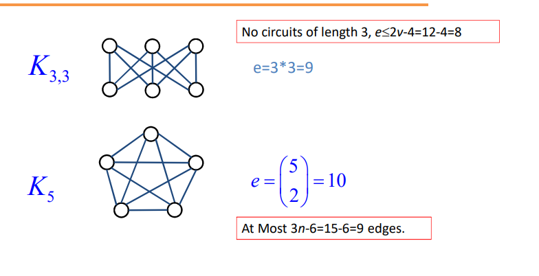
If a connected planar simple graph has edges and vertices with and no circuit of length three, then
Kuratowski Theorem
Kuratowski Graph
Kuratowski graphs are two typically non-planar graphs.
In the Kuratowski graph, we can find that:
- If we replace edges in a Kuratowski graph by paths of whatever length, they remain non-replace.
- If a graph contains a subgraph obtained by starting with or and replacing edges with paths, then is non-planar.
Homeomorphic Graph
If a graph is planar, so will be any graph obtained by removing an edge and adding a new vertex with edges and . Such an operation is called an elementary subdivision .
The graphs are called homeomorphic if they are obtained from the same graph by a sequence of elementary subdivisions.
Kuratowski Theorem
A graph is planar if and only if it contains no subgraph obtained from or by replacing edges with paths.
Graph Coloring
Lead in: four colors are always enough to color any map drawn on a plane.
Coloring graphs
Suppose that is a graph without no multiple edges, and is any set of colors. Any function is called a coloring of the graph using colors.
A coloring is proper if any two adjacent vertices and have different colors. The smallest number of colors needed to produce a proper coloring of a graph is called the chromatic number of , which is denoted by .
Four-color Theorem
The vertices of ant planar graph can be 4-colored in such a way that no two adjacent vertices receive the same color.
This is hard to prove.
Five-Color Theorem
Any planar graph can be colored with five colors.
Prove
Let be a node-minimal counter-example to the theorem, for example, a planar graph that requires 6 colros.
As is a planar graph, we can get must have a node with degree . Let the nodes adjacent to q be named as , and this five nodes can not form , also because this is a planar graph. So there must be two vertices in this five vertices that have no edge between them.
So we can "contract" the edges and to get a new planar graph , and the vertices , and become a new vertices in . is 5 colorable since it has fewer nodes than , so we can find that we color the using the five colors in the , which meaning the counter example is not counter.
Applications of Graph Coloring
- Fifteen different foods are to be held in refrigerated compartments within the same refrigator.
- How can the final exams be scheduled at a university so that no students has two exams at the same time.
- Frequency assignment. we need to assign different radio frequency to two radio station whose distance is to short.
Chromatic Polynomials
If is a graph and is an integer, let be the number of ways to color properly using or fewer colors. is called the chromatic polynomials. And if we can find the chromatic polynomials ,we can easily get the chromatic number of .
For example, for a linear graph , we have the chromatic polynomials , so , and , so .
Theorem 1
If is disconnected graph with components , then is the product of the chromatic polynomials for each components.
Subgraph and Quotient Graphs
One of the most important subgraphs is the one that arises by deleting one edge and no vertices. If is a graph and , then we denote by the subgraph obtained by omitting the edge from and keeping all vertices.
Suppose that is a graph without multiple edges between the same vertices and that is an equivalence relation on the set . Construct the quotient graphs as follow: The vertices of are the equivalence classes of produced by . If and are the equivalence classes of vertices and , then there is an edge in from to if and only if some vertices in is connected to sone vertices in in the graph .
Theorem 2
Let be a graph without multiple edges, and let , say . So we have , subgraph obtained by deleting and , the quotient graph of obtained by merging the end points of . And then with colors:
Transport Networks
An important use of labeled graph is to model what are commonly called transport networks. The label on an edge represents the maximum flow that can be passed through that edge and is called the capacity of the edge.
Transport Network
A transport network, or a network, is a connected digraph with the following properties:
- There is a unique node, the source, that has in-degree 0. We always label the source with node 1.
- There is a unique node, the sink, that has out-degree 0. If has n nodes, and we always label the sink with node n.
- The graph is labeled. The label, , on edge is a nonnegative number called the capacity of the edge.
Flow
A flow in a network is a function that assigns to each edge of a nonnegative number that does not exceed .
And when talking about flow, we have:
- Conservation of flow
- Value of flow
For any network, an important question is to determine the maximum value of a flow through the network and to describe a flow that has the maximum value.
Although edge is not in , there is no harm in consideration such a virtual flow as long as it only has effect of reducing the existing flow in the actual edge )
Labeling Algorithm
Let be a network with nodes and be the symmetric closure of . All edges and paths used are in .
- Begin with all flows set to 0.
- As we proceed, it will be convenient to track the excess capacities in the edges and how they change rather than tracking the increasing flows.
- When the algorithm terminates, it is easy to find the maximum flow from the final excess capacities.
STEP 1
- Let be the set of all nodes connected to the source by an edge with positive excess capacities.
- Label each node in with , where is the excess capacity of edge . The 1 in the label indicates that is connected to the source, node 1.
STEP 2
-
Let node in be the node with the smallest node number and let be the set of all unlabeled nodes,
other than the source and those are joined to node and have positive excess capacity.
-
Suppose that node is in and is the edge with positive excess capacity. Label node with , where is the minimum of and the excess capacity of edge .
-
When all the nodes in are all labeled in this way, repeat this process for the other nodes in . Let
STEP 3
-
Repeat Step 2 , labeling all previously unlabeled nodes that can be reached from a node in by an edge having positive excess capacity.
-
Continue this process forming sets , , ... until after a finite number or steps
-
either the sink has not been labeled and no other nodes can be labeled. It can happened that no nodes have been labeled; remember that the source is not labeled or the sink has been reached.
In this case, the algorithm terminates and the total flow is a maximum flow.
-
or the sink has been labeled.
In this case, the sink has been labeled with where is the amount of extra flow that can be made to reach the sink through the path.
STEP 4
We examine the path in reverse:
- If edge , we increase the flow in and decrease the excess capacity by the sam amount. Simultaneously, we increase excess capacity of the virtual edge
- If on the other hand , edge , we decrease the flow in and increase its excess capacity. Same as before, decrease the excess capcaity in .
Back to the step 1.
What a complex algorithm!
Cut
A cut in a network is a set of edges having the property that every path from the source to the sink contains at least one edge from .
The capacity of a cut is the sum of the capacities of all edges in . If is any flow and is any cut, there must be .
And we have a theorem that a maximum flow in a network has value equal to the capacity of a minimum cut of the network.
Super Source & Super Sink
When we meet a network with sources or sinks more than one, we can add a virtual source or virtual sink to use the labeling algorithm, which is connected with the real source and sink with large enough edge. These virtual source and sink is are called super source and super sink.